The logistic function revisted

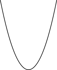
Today we revisit one of our most popular articles, on the logistic function:

f(x) = ax(x-1)

In the original article, we demonstrated how we can use this function as a “logistic map” by iterating (i.e.,applying it repeatedly to the previous result). The logistic map produced different sorts of behavior depending on the values of a. For example, for some values of a, iteration settles into a cycle, bouncing among two or more points on the function.

The original article provided more examples and more detail about the mathematics, and those who are interested are encouraged to go back and check it out. One of the main this we discussed was how one can characterize the logistic function over
different values of a using a graph called a bifurcation
diagram
. As the values of a increase (a is labelled as “r” in this graphic I shamelessly but legally ripped off from wikipedia), one can observe vertically the period doubling where the logistic map converges on a single value, then bounces between two points, then four, then eight, and so on, until the onset of chaos at approximately 3.57.

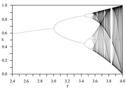
When a is greater than or equal to 4, the function “diverges”, i.e., it just gets bigger and bigger (or smaller and smaller because the numbers are negative) when you repeatedly apply it.

The bifurcation diagram shows what happens for real values of a, i.e., all integers, fractions and other numbers that can be expressed as a decimal. But suppose we allow a to be any complex number, or any combination of real and “imaginary” numbers (i.e., square roots of negative numbers). Real numbers can be expressed a line, while complex numbers are expressed on a plane. So we can produce an analog of the bifurcation diagram over a plane instead of a line as above.

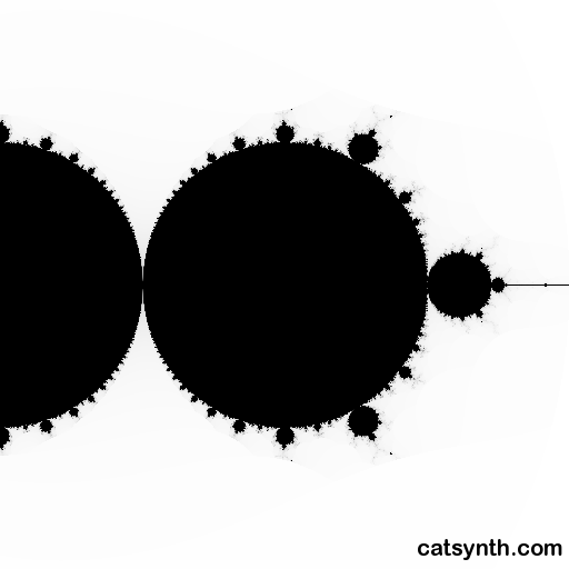
In the following diagrams, we are looking at the complex plane of
different values for a. If the logistic map converges to either a single value or a cycle, the location on the plane is colored in black. If it diverges, i.e., gets infinitely farther away from zero, then the location is white. Unlike for real numbers, where the convergent “black” values of a form a simple line segment, for complex numbers the set of convergent values is a lot more “complex”:

Zooming in, we can see the structure of the set, with lots of smaller “bubbles” and “filaments” off of the main circles. The large circles are the complex-number equivalents of the single-line sections of the bifurcation diagrams, with the small bubbles representing cycles and period doubling.

Some readers might recognize similarities between this set and more well-known Mandelbrot set:

The similarity is more than coincidence, as the Mandelbrot set is based on a map similar to the logistic map. But the Mandelbrot set has the pronounced cardioid shape and asymmetry different from the logistic-map set. Zooming in further, we see that filaments and local areas of the two sets have more similarity. Indeed, we see small “Mandelbrot-like sets” at the junctions of the filaments:

It is interesting how these miniature versions have a shape similar to Mandelbrot set rather than the double-circle of the logistic-map set.

Although these sets have a “fractal-like” qualities, neither is a fractal in the strict sense of the word. They are not strictly self-similar, nor do they have fractional dimension. Nonetheless, we are featuring the logistic-map set as a “Friday Fractal” , an event started by our friend Andrée at meeyauw.

I am not sure the logistic-map set has a name like the Mandelbrot set has, so how about calling it the CatSynth set?

Submitted to Carnival of Mathematics #29.


New Podcast: "Bi-fur-cation" demo


Click here to listen or subscribe.

Some might consider tonight's podcast a “rerun” of sorts, as this musical example was featured in the CatSynth article The Logistic Function and its Discontents. This is actually one of our most popular articles of our stats/records are to be trusted, combining mathematics, the work of Antoni Gaudí, and some of my favorite electronic-music techniques. Those who have not read the article are encouraged to do so – I hope to post a follow-up one of these days. Or you can just listen to the podcast as a musical curiousity.

The Logistic Function and its Discontents

This article explores the mathematical and more specifically the musical products of a very simple equation. In that exploration, we touch not only mathematics and music, but art, architecture, nature and philosophy; so those who are usually squeamish about mathematics are encouraged to read on.

Most readers who made it through high school algebra should be familiar with quadratic functions and the parabolas described by these functions on the x-y plane. For those who have forgotten, a parabola looks like this:

Parabolas are seen not only in high-school math classes, but often in nature as well. Among the most exquisite uses of parabolae can be found in the architecture of Antoni Gaudí. I had the priveledge of seeing many of his buildings and spaces in Barcelona, including this magnificent example of parabolic architecture:

But (as usual), I digress. For the remainder of this article, we will focus on a particular class of these functions, called logistic functions:

f(x) = ax(x-1)

Logistic functions have roots and 0 and 1, and describe a downward facing parabola (or “water-shedding parabola” in the parlance of my high-school pre-calculus teacher). The peak of this parabola depends on the value of a, and as we will soon see, this is the least of the interesting properties dependent on a.

Now, instead of simply graphing the function on an x-y plane, apply the output of the function back as the next input value in a process known as iteration:

xn+1 = axn(xn1)

This is a fancy way of saying “do the function over and over again.” What is interesting is that for different values of a, one will get different results. For low values (where a is less than one), repeated iterations get closer and closer to zero. If a is between 1 and 3, the it will end up at some value between zero and one. Above 3, things get more interesting. The first range bounces around between two values, as characterized below:

As a increases, eventually the results start bouncing among four values, and then eight, then sixteen, and so on. These “doubling periods” get closer and closer together (those interested in this part of the story are encouraged to look up the Feigenbaum constant). Beyond about 3.57 or so, things get a little crazy, and rather than settling into a period behavior around a few points, we obsserve what is best described as “chaotic behavior,” where the succession of points on the logistic function varies unpredictably.

It is not random in the same way that we usually think of (like rolling dice or using the random-number generators on our computers), but has rather intricate patterns within – those interested in learning more are encouraged to look up “chaos.” This chatoic behavior can be musically interesting, and I have used the chaotic range of the logistic function in compositions, such as the following except from my 2000 piece Spin Cycle/Control Freak.

One can more vividly observe the behavior I describe above as a graph called a bifurcation diagram. As the values is a increase (a is labelled as “r” in this graphic I shamelessly but legally ripped off from wikipedia), one can oberve vertically the period doubling where the logistic map converges on a single value, then bounces between two points, then four, then eight, and so on, until the onset of chaos at approximatley 3.57.

There are tons of books and online articles on chaos, the logistic function, and its bifurcation diagram. Thus, it’s probably best that interested readers simply google those phrases rather than suffer through more of my own writing on the topics. However, I do have more to say on my musical interpretations of these concepts.

Given my experience in additive synthesis and frequency-domain processing (if I have lost you, then skip to the musical excerpt at the end, it’s pretty cool), I of course viewed this map as a series of frequency spectra that grow more or less complex based on a. I implemented this idea in Open Sound World. using the logstic function and its bifurcation diagram to drive OSW’s additive synthesizer functions. The results were quite interesting, and have been used in several of my live performances. I use my graphics tablet to sweep through different values of a on the horizontal axis as in the bifurcation diagram:


Photo by Tiffany Worthington

The resulting sound is the synthesis of frequences based on the verticle slice through the diagram.

Click here to listen to an example.

In the periods of chaos, the sound is extremely complex and rich. Below 3.57 and in the observable “calm periods,” the sound is simpler, containing on a few components forming somethin akin to an inharmonic chord. In true chaotic fashion, small movements along the horizontal axis result in dramatic differences in the spectrum and the timbre. The leads to a certain “glitchy” quality in the sound – one can practice control over time to make smooth transitions and find interesting “islands of stability” within the timbral space.

I have used this simple but evocative computer instrument in several performances, including my 2006 Skronkathon performance as well as my work last year with the Electron SAlon series. I have really only scratched the surface the possibilities with this concept, and hope to have more examples int the future.